What the radio taught me about Deep Learning

During one of the courses I was following on Coursera, Andrew Ng mentioned that using the activation function was key to the success of deep learning methodologies. At that time, I didnt understand why. For some reason I was also simultaneously thinking about the FM radio circuits (perhaps it was something that I was reading about online). And then it hit me - the two are practically identical. In this blog, I typed out my thoughts.

1. A Deep Net without activation is a Logistic Regressor

Let us consider a first layer of the network. The input is a vector \(\mathbf{x}\), with associated weights matrix \(\mathbf{W}_1\) for the first layer (we shall neglect the bias term which, will not change the mathematics too much). At the end of the first layer, the output values (\(\mathbf{x}_1\)) are simply:

$$\mathbf{x}_1 = \mathbf{W}_1 \mathbf{x}$$

This goes to the second layer, which has weights \(\mathbf{W}_2\). Once these weights are applied, to the output of the first layer, the output of the second layer is then given as:

$$\mathbf{x}_2 = \mathbf{W}_2 \mathbf{x}_1 = \mathbf{W}_2 \mathbf{W}_1 \mathbf{x} = \mathbf{W}_{21} \mathbf{x}$$

where, \(\mathbf{W}2 \mathbf{W}_1\) is represented by the single matrix \(\mathbf{W}{21}\) . We can continue this process for the rest of the layers of a neural network. Or, we can stop here. The final result is a linear model.

2. Revisiting the simple diode mixer

The mathematics of the FM radio is revolves around the idea of a nonlinear mixer. Any nonlinear circuit can mix signals - even the unassuming diode. When the external signal \(V_{RF}\) and the the signal from the local oscillator \(V_{LO}\) is passed through a diode, it mixes them to form higher-order harmonics. Take the example of the simplest unbalanced mixer shown below:

The result of the intermediate frequency voltage \(V_{IF}\) is proportional to the current through the diode \(I_D\) as:

$$I_D = I_0 \Big( \exp \big( \frac {qV_D} {nkT} \big) - 1 \Big)$$

Since the exponential is a non-linear function, it can be expanded into its series form:

$$\Big( \exp \big( \frac {qV_D} {nkT} \big) - 1 \Big) \approx x + \frac {x^2} {2} + \ldots$$

So what happens when the two signals are applied to the circuit above?

$$\frac {I_D} {I_0} \approx \Big( \frac {q (V_{RF} +V_{LO})} {nkT} \Big) + \frac {1} {2} \Big( \frac {q (V_{RF} +V_{LO})} {nkT} \Big)^2 + \ldots$$

You will notice that the expansion of the higher-order term in the nonlinearity is what allows for the mixing of the signals. Frequency modulation is essentially a result of this mixing, and the result of some more trigonometry. The trigonometry isn’t very interesting to us at the moment. What is important to realise is that the nonlinearity produces the higher-order terms …

the nonlinearity produces the higher-order terms …

3. A neuron with \(\tanh\) activation

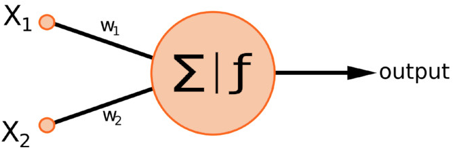
Let us now take a look at a perceptron:

(Photo credit: https://www.simplicity.be/article/machine-learning-in-web-games/)

3.1. Adding activation to a linear regressor

When a nonlinear function is added to the end of a regressor, exactly the same phenomenon occurs. Let us say for example, that the activation used in the diagram above happens to be a \(\tanh\)-type activatio. \(\tanh(W_1X_1 + W_2X_2)\). This result by itself in rather uninteresting. However, consider what it means for the input to have nonlinearity in the input. The expression may be approximated in the form of Taylor series, as shown in the next Section.

3.2. The \(\tanh\) taylor series expansion

Let us remind ourselves of the \(\tanh\) Taylor series expansion.

$$\tanh(x) = x - \frac {1} {3} x^3 + \frac {2} {15} x^5 - \ldots$$

Here, even if we just consider the first two terms, we notice that the activation from a two-input neuron takes the form:

$$\tanh(W_1X_1 + W_2X_2) = (W_1X_1 + W_2X_2) - \frac {1} {3} (W_1X_1 + W_2X_2)^3 + \ldots$$

which when expanded, produces all manner of higher-order features.

4. Conclusion

Activated neurons \(\approx\) logistic-regression with higher-order features, only better. The result of activations in neural networks is simply to generate a set of highly nonlinear combinations of parameters. If we indeed think of the neural network as a nonlinear form of the regressor/classifier, all mathematics developed for the linear regressor (with added nonlinear features) can be immediately carried forward to the neural network.

Activated neurons \(\approx\) logistic-regression with higher-order features, only better.

One of the important considerations in such cases would be the bias-variance conundrum that data scientists face on a regular basis. Similar problems in linear models are typically solved by L1 and L2 regularization (or a combination of the two - the Elastic Net). Similar methods, then, should hold for regularizing neural networks as well. I’ll explore this in the next article.

From a philosophical point of view, early attempts at generating neural networks were an attempt at replicating the way in which the brain works. It is surprising that neural network appears to be an elaborate representation of linear models with higher-order features. Under such circumstances, it is also worth noting that traditionally linear models have been viewed as “easy-to-understand,” while neural-network models have been viewed as “black boxes”. This interpretation should assuage fears of using neural network models stemming from the black box interpretation.

Further Reading

For further reading, the following information might help

• Diode mixer